EEGLAB Home
May, 2012: Version 1.00
- What is CIAC?
- Requirements
- Download and Installation
- Tutorial
- Citing CIAC
- Licence
- References
- Acknowledgements
CIAC plug-in is a set of Matlab functions written by Filipa Campos Viola, which allows the identification and clustering of independent components (ICs) representing cochlear implant (CI) artifacts. This tool is based on temporal and spatial properties of the ICs and uses three user-defined threholds to find those ICs that represent cochlear implant artifacts. CIAC is designed to work within the EEGLAB environment, providing a GUI to identify and cluster artifactual ICs across subjects. All functions can also be used from the Matlab command line, providing expert users with the ability to use them in custom scripts.
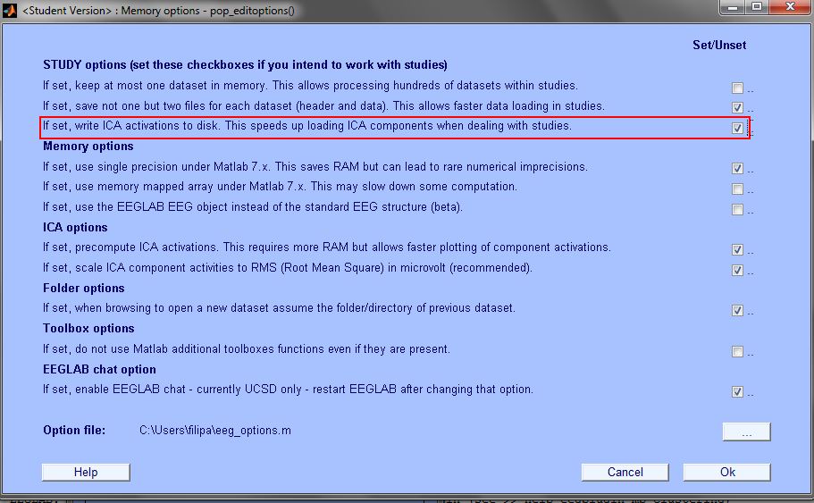
In addition to the requirements of EEGLAB, CIAC plug-in needs the Matlab Statistics Toolbox to work. It is also mandatory that you have run ICA for all datasets that you want to use, as well as the DIPFIT plugin. We also recommend that common biological artifacts, such as eye blinks or heartbeat should have been previously corrected from all datasets. ICs from
one or more EEG dataset, epoched to the same auditory stimuli of
interest. A STUDY set must then be created using these datasets. Please note that the field EEG.icaact is mandatory. Before loading your STUDY set please select the adequate "Memory and other options". Please see below.
1) Download the compressed CIAC plug-in file ciac1.00.rar into your 'plugins' directory of your EEGLAB
distribution.
2) Uncompress the donwloaded file using utility software. Inside your 'plugins' directory, you should now have a directory called 'ciac1.00.zip' containing all the necessary m-files and binaries and a pdf with the reference paper. Starting EEGLAB should now automatically recognise and add the plug-in.
You should see the following line appear in your Matlab environment window: That's it.
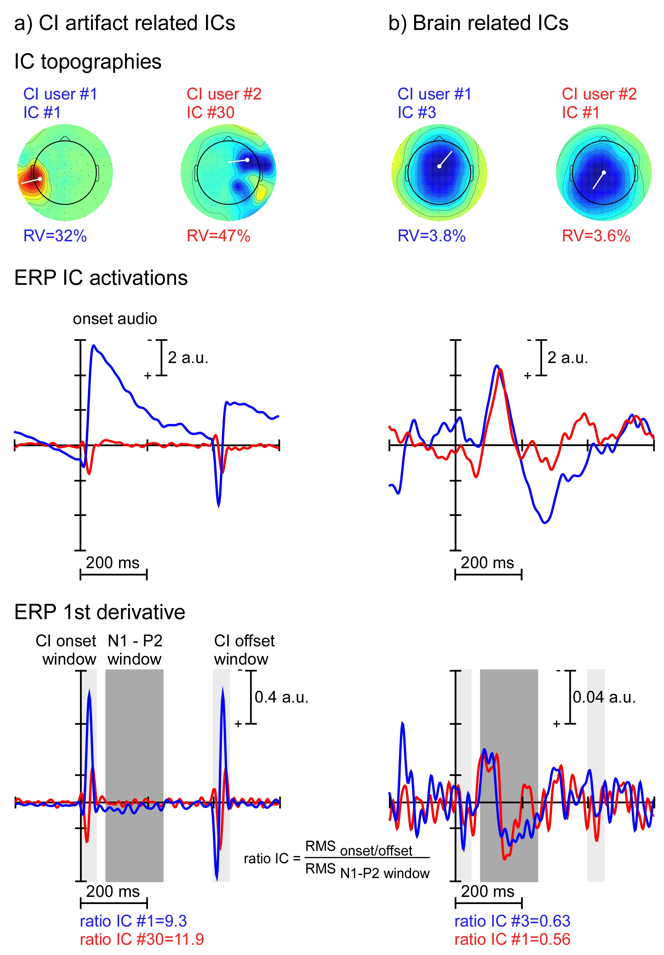
This short tutorial will take you through using CIAC from the GUI. We will show you how to get started in a few steps. We encourage you to try following these steps using your own data and adjusting the thresholds. We will also assume that you know the basics of EEGLAB e.g. loading a dataset, creating a study set, plotting, data structures, etc. If not, refer to the EEGLAB website for more information. It is also important that you are familiar with the properties of ICs representing CI artifacts, as well as the outputs provided by the DIPFIT plugin. Very briefly, this tool computes the equivalent dipole source localization of independent components. For more details please see DIPFIT documentation. Fig. 1. Properties of independent components (ICs). Column a) shows two ICs representing the cochlear implant (CI) artifact for user #1, implanted on the left side, (blue) and user
#2, implanted on the right side (red). Column b) shows another two ICs representing brain related activity for the same CI users. The top row shows the ICs topographies and the
respective residual variance (RV) in % after dipole fitting. 2-D projections of dipole location and orientation are indicated in black on top of the topographic maps. The middle row
shows the ERP of each IC activation. Zero ms represents auditory onset and amplitude values are expressed in arbitrary units (a.u.). The bottom row shows the temporal derivative of
the ERP for each IC. The time windows corresponding to the onset of the CI artifact are displayed in light gray, whereas the time window representing activity of interest (N1-P2
peaks) is displayed in dark gray. For each IC the ratio between the root mean square (RMS) amplitude in the onset/offset window and the RMS amplitude in the time window of
interest was calculated (ratio IC). For more details please read CIAC paper [1].
2) Loading a STUDY set and open CIAC
eeglab: adding "ciac1.00" plug-in (see >> help eegplugin_ciac)
1) Properties of independent components (ICs)
The figure below summarizes the properties of ICs represeting CI artifacts..
Load a study set (File > Load existing study).
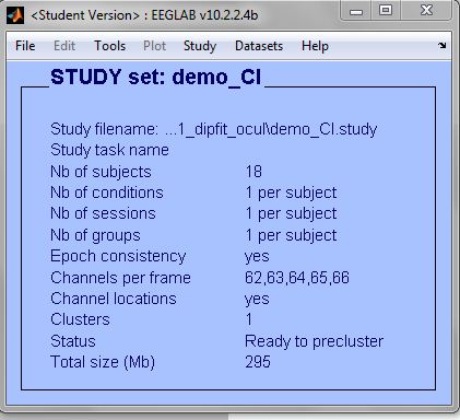
In our example the study set is called: 'demo_CI.study'. It is constituted by 18 datasets.
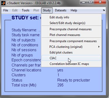
The following menu is displayed.

3) Editing input parameters
There are seven parameters that can be changed by the user. Please note that all parameters are mandatory. Before showing how to run CIAC using the study selected above, we briefly describe the input parameters.
Duration of auditory stimuli: Must be a value in miliseconds corresponding to the duration of the auditory stimuli used in the experiment.
Time window AEP: The time window of interest for the AEP response needs to be defined as an interval in miliseconds. Example corresponding to N1-P2 latency window: [80 to 250].
Threshold RV (thr-rv): This threshold is based on the outputs from the DIPFIT plugin. The residual variance (RV) between the actual IC topography and the model projection for the equivalent dipole to the same electrode montage can be used as a differentiation criterion, since brain related ICs are dipolar and thus have a much lower RV. This is then an exclusion step to avoid the further selection of ICs that would likely represent brain related activity. Values below 0.25 are recommended for this threshold.
Threshold derivative (thr-dev): This threshold is related to the ratio IC described in fig. 1 (please see above). The recommended
values are between 1.5 and 3.5. This range is motivated by a previous study [2] where the ICs manually labeled as CI artifact were characterized by a ratio range between 1.5 and 12. For more details please check CIAC reference paper [1].
Threshold correlation (thr-corr): Based on the previous threshold (thr-dev) an IC is selected as the most likely to represent the CI artifact. Its topographical map is then correlated to the maps of the other ICs. For this threshold the recommended values are between
0.85 and 0.95, which represents a rather conservative
range, since in our experience ICs reflecting CI artifact have either very similar or uncorrelated topographies.
Index from channel of interest: The user can select the channel where the maximum AEP response is expected. This information will be used when creating the output plots. It will help to evaluate the level of correction that can be achieved.
Display output plots: This option allows either inspecting the output plots after single dataset processing ("display plot=1") or saving the figures in .tiff format in the same folder where the STUDY set is stored ("display plot=0"). In the first case after processing the first dataset the computation is paused and three output plots are displayed. The user has the opportunity to inspect the outputs on the fly. When the user has finished the inspection, he/she can press any key and the computation for the following dataset will be initiated. In the other case the computation will run without pauses and all output plots for all datasets will be stored and can be inspected later. In this case the only output displayed is the grand average AEP plot for all datasets contained in the STUDY set. The output plots are described in the next section.
IMPORTANT: Please note that a set of
thresholds needs to be defined only once. The set of thresholds depends only on the type and duration of auditory stimuli used and is not related to the type of CI device. The set of thresholds chosen is applied always to all datasets comprised in a study set.
4) Running CIAC using the demo study set
In the CIAC menu we insert the following information for the seven mandatory parameters.
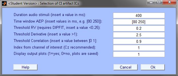
After entering the values for the parameters, we press 'OK'.
While CIAC is processing the data, a number of info messages are displayed in the command line. Here is an example:
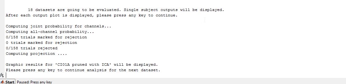
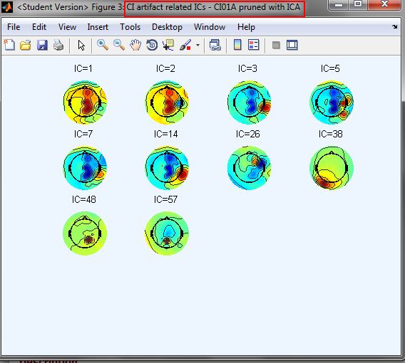
Please note that the computation is paused because we selected "display plot=1". The outputs for the first dataset are displayed. The first output figure shows the topography plots of the components suggested as representing the CI artifact. On the top of each plot, the respective IC index is displayed. Note that the name of the corresponding dataset is shown on the top.
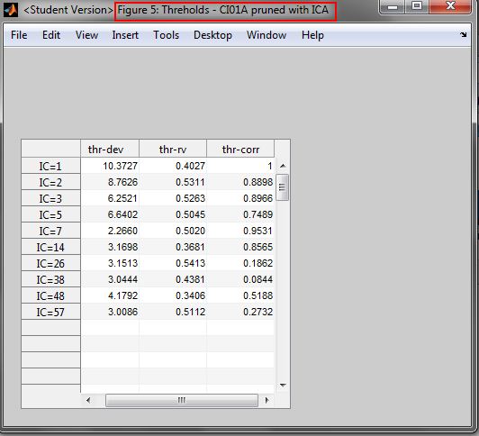
Next a table is displayed showing the three thresholds for each of the suggested ICs.
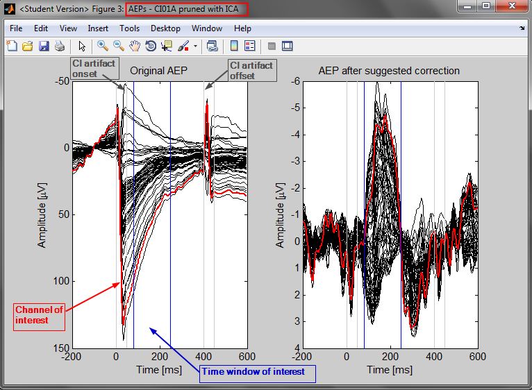
The third output shows the original AEP (left) and the AEP that can be obtained after correction of the suggested ICs (right). Note that the time window of interest is highlighted in blue. Note that the time windows corresponding to the onset and offset of the CI artifact are also shown (gray). The channel of interest is shown in red. In this example it corresponds to Cz.
.
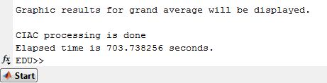
After inspecting the output plots, the user should press ENTER, so the computation will continue and the outputs for the next dataset can be evaluated. When CIAC finishes computing all datasets, the following message is displayed in the command line.
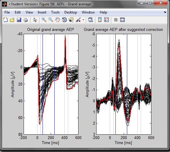
A summary plot is then displayed showing the original grand average AEP (left) and the "corrected" grand average AEP (right).
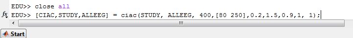
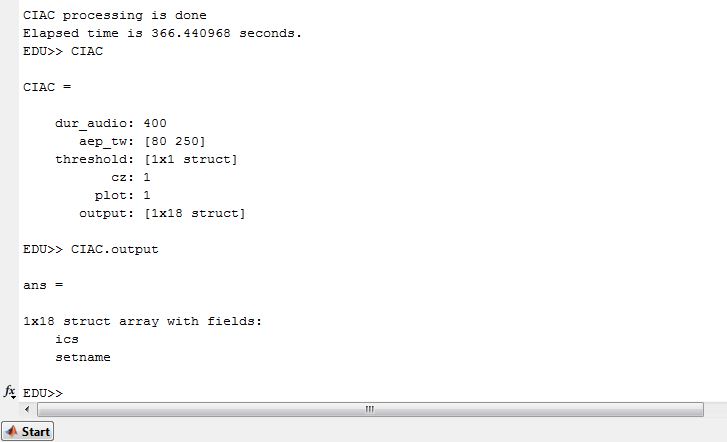
Note that when using CIAC from the GUI only graphical outputs are available. If you would like to store the indices of the ICs suggested as representing the CI artifact you need to run the tool from the command line. Please see an example below.
.
The output of the tool is a structure called CIAC and contains six fields. The first five fields store the input parameters selected by the user. The field CIAC.output contains two sub-fields where the indices of the ICs suggested as representing the CI artifact are stored for all evaluated datasets. Please see below.
This concludes the tutorial. If you would like to learn more about other CIAC features, please read CIAC paper [1].
This is a free software distributed under the GPL. However, the authors do ask those that find this program of use to cite it in their work refering to [1]. Also, please make sure that EEGLAB is cited properly as described in the EEGLAB website.
The CIAC plug-in functions, sources and programs are released under the terms of the GPL.
CIAC plug-in is distributed "AS IS" under this Licence in the hope that it will be useful. The authors make clear that no condition is made or to be implied, nor is any warranty given or to be implied, as to the accuracy of the Software, or that it will be suitable for any particular purpose or for use under any specific conditions. Furthermore, the authors disclaim all responsibility for the use
which is made of the Software. They further disclaim any liability for the outcomes arising from using the Software.
By downloading or making this software available to others you agree to the terms of this licence and agree to let these terms known to other parties to whom you make this software available.
[1]Viola FC, et al. Semi-automatic identification of cochlear implant artifacts for the evaluation of late auditory evoked potentials. Hear Res. 2012, Feb; 284(1-2): 6-15.
[2]Viola FC, et. al. Uncovering auditory evoked potentials from cochlear implant users with independent component analysis. Psychophysiology. 2011, Nov; 48(11):1470-80.
This work was partially supported by Fundacao para a Ciencia e Tecnologia, Lisbon, Portugal (SFRH/BD/37662/2007) to Filipa Campos Viola. Major technical advises were provided by Stefan Debener, Jeremy Thorne and Maarten De Vos. We also thank Pascale Sandmann for additional testing.
This page was last updated May 20, 2012.